Understanding Stochastic Outlier Selection

utliers are data points/observations which defect or diverge from the general pattern. In this article, we will implement the Stochastic Outlier Selection Algorithm for Pseudo Dataset. The dataset will be generated with two features and hence the outlier here will be multivariate (i.e. Having or involving multiple variables). The SOS algorithm is an unsupervised outlier selection program. It was fashioned and engineered by Jeroen Janssens and his publication (https://research.tilburguniversity.edu/en/publications/77b71572-7266-44d0-9510-ebf4eeb43062) here details the algorithm, its implementation. All references and justifications and understanding was developed from the cited paper. This article attempts to implement that SOS algorithm. Following is my GitHub Repository of the code below: https://github.com/AmanPriyanshu/py-stochastic-outlier-selection/blob/master/SOS_outlier_detection.ipynb

DATASET:

We will be generating our own dataset since this is an implementation-oriented article. We will evaluate this dataset and look at potential use cases for this algorithm following our implementation.

Defining our dataset: Our data will consist of 50 points plotted in 2-D space. They will be generated using the following:

This will generate us a list of fifty 2-D points, this we can use as data. As we can see most of the points will be closely linked to each other as they are restricted within the range 0 to 100. However, some points precisely 5 will be an outlier as they will deviate from the general trend.

Let us see the plot of any such instance of the data.

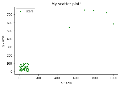
We can clearly differentiate between the cluster and outliers here. Now let us begin with normalizing this dataset. Normalization is a technique often applied as part of data preparation for machine learning. The goal of normalization is to change the values of numeric columns in the dataset to a common scale, without distorting differences in the ranges of values. Thereby, any feature which inherently has large values will not bias or over-influence the clustering algorithm. Normalization will be enacted using the code:

Once this data is normalized we are ready to begin our clustering algorithm.

CLUSTERING:

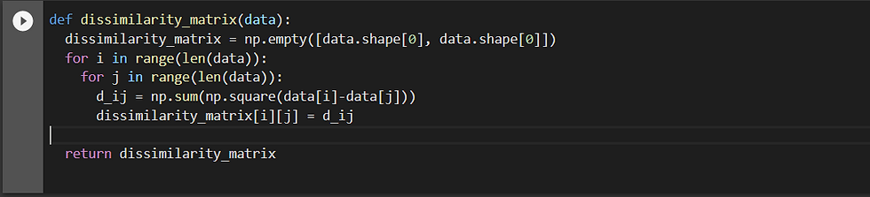
Step 1: DISSIMILARITY MATRIX:

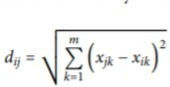
A dissimilarity matrix is one where the euclidean distance of each point w.r.t. every other point is generated it is done feature-wise and then per data-point is simply summed.

It is given by the following formula:

It is implemented in the following manner:

Once Calculated the dissimilarity matrix gives us the euclidean distance of all the points w.t.r. to each other. For example for the dataset:

The dissimilarity matrix is:

Now here take a look at the first and the last row, the first row being an outlier has most of its distance greater than 0.9 breaking the sequence with a 0.08 when another outlier is compared. Similarly, the last row which has an index 49 is a normal case. Therefore, most of its distance is very low even below 0.01, however, when compared to an outlier such as the first datapoints it gives a value greater than 1 (Eg: 1.613 when compared to first data-point). This is the importance of the distance matrix, it highlights all points w.r.t. each other.

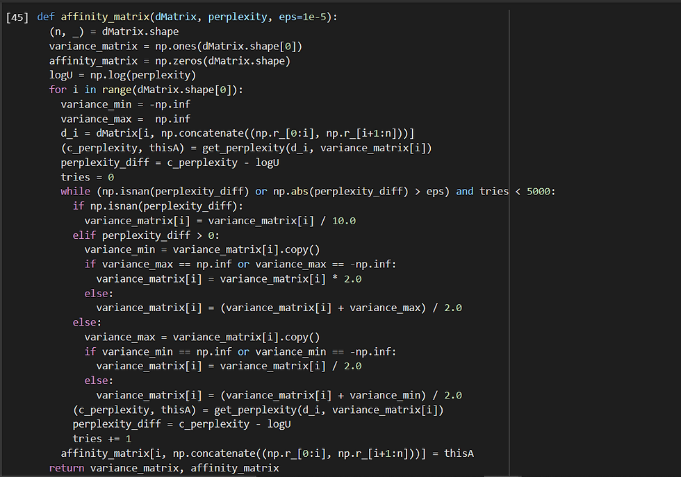
Step 2: AFFINITY MATRIX

Now let us create the affinity matrix the most important part of SOS. Here we employ affinity in order to quantify the relationship from one data point to another data point.

We note that the affinity that the data point x[i] has with data point x[j] decays Gaussian-like with respect to the dissimilarity d[i][j], and a data point has no affinity with itself, i.e., a[i][i] = 0.

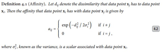
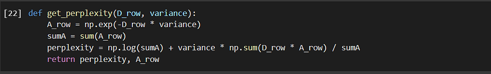
The value of each variance σ2[i] is determined using an adaptive approach such that each data point has the same number of effective neighbours, i.e., h (perplexity). The adaptive approach yields a different variance for each data point, causing the affinity to be asymmetric. Now, here the perplexity parameter h can be compared with the parameter k as in k-nearest neighbours, with two important differences. First, because affinity decays smoothly, ‘being a neighbour’ is not a binary property, but a smooth property. Now we need to adapt the variance in such a way that the perplexity is the same for every row. We take perplexity = 25 here. Therefore, the implementation of it in code:

and

Let us take a look at the output of the first (outlier) and last (normal) row/data-point:

affinity_matrix:

Take a look at the first row which is an outlier. Here, we can see that the outlier has low values for every normal case it is in the order of 0.1 or 0.2 generally. However, any other outlier has a value near 0.9 or 0.8. On the other hand, the last row which is a normal data-point has a very very low affinity towards outlier even equal to e^-196 in some cases. Whereas, all normal cases have a value greater than 0.5 even in the range of 0.5 to 0.7.

Step 3: BINDING MATRIX:

The binding matrix is a row-wise normalized version of the affinity matrix. It is given by the following code:

Now let us take a look at the matrix it gives as output:

Taking a look at the first row (which is an outlier) we can see that most of the values are of the order of 0.01 on the other hand upon outlier data-point it is in the order of 0.07. In the case of a normal data-point, we can see that normal-points are of the order 0.01 or 0.02 and outliers are very low even to the order of e^-100. This clearly highlights the value of the binding matrix which allows us to analyse the bound-affinity of all the data-points w.r.t. each other.

Step 4: OUTLIER PROBABILITY MATRIX:

Now, the probability matrix gives us the probability of whether a particular data-point is an outlier or not. It is given by the mathematical formula:

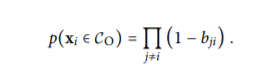
Here we can clearly see that what we are attempting to do is we are calculating the product of the probability with which data-point[i] is not a neighbour of data-point[j] where j ranges from 0 to n-1 except i. But since j=i will anyways give us (1-0.0) it outputs 1 and hence does not affect the probability that a particular data-point is an outlier or not.

The code implementation is given by:

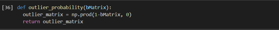
Let us take a look at the output, as this is the final probability of whether a data-point is an outlier or not:

Now take a look here, we can see the different probabilities with which a particular data-points are an outlier or not. We can see that the first point is an outlier with the probability of 73.83% whereas the second is an outlier with a probability of only 34.92% and hence we can conclude that it is not an outlier but rather part of the cluster. We can create an if-condition where every data-point having a probability above 70% is categorised as an outlier.

Step 5: CLASSIFIER:

We can represent the output as:

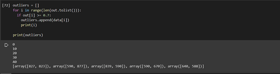
We can clearly see the accuracy of the SOS algorithm with the only parameter to set up being perplexity (used: 25, here).

CONCLUSION:

SOS is a very useful outlier selection algorithm and it has far superior performance than 1) KNNDD 2)Outlier-score plots 3)LOF 4)LOCI 5)LOCD. It is clearly a very useful outlier selection algorithm and can be used in many different datasets.